Fast Fourier Transforms

Description

A physical process can be described either in the time domain, by the values of some quantity h as a function of time t, e.g., h(t), or else in the frequency domain, where the process is specified by giving its amplitude H as a function of frequency f, that is H(f), with

. For many purposes it is useful to think of h(t) and H(f) as being two different representations of the same function. One can go back and forth between the two representations by means of the Fourier transform equations,

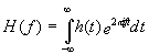and

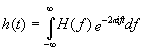
FFT is a fast (computationally efficient) way to calculate the Discrete Fourier Transform. Functionally, the FFT decomposes the set of data to be transformed into a series of smaller data sets to be transformed. Then, it decomposes those smaller sets into even smaller sets. At each stage of processing, the results of the previous stage are combined in a special way. Finally, the DFT of each small data set is calculated. e.g. an FFT of size 32 is broken into 2 FFT’s of size 1, which are broken into 4 FFT’s of size 8, which are broken into 8 FFT’s of size 4, which are broken into 16 FFT’s of size 2. Calculating a DFT of size 2 is trivial.
It turns out that it is possible to take the DFT of the first N/2 points and combine them in a special way with the DFT of the second N/2 points to produce a single N-point DFT. Each of these N/2-point DFTs can be calculated using smaller DFTs in the same way. One (radix-2) FFT begins, therefore, by calculating N/2 2-point DFTs. These are combined to form N/4 4-point DFTs. The next stage produces N/8 8-point DFTs, and so on, until a single N-point DFT is produced.
The DFT takes

operations for N points. Corresponding FFT takes Nlog₂(N).

Algorithms

Double Precision FFT of Vector of Complex Numbers

The Fourier transform is calculated as:

where X is the input vector of double precision complex numbers and A is the output vector of double precision complex numbers.

The Inverse Fourier Transform is calculated as:

2-D Double Precision FFT of a Matrix of Complex Numbers

The Fourier transform is calculated as:

where X is the input matrix of double precision complex numbers and A is the output matrix of double precision complex numbers.

The Inverse Fourier Transform is calculated as:

Double Precision Sine or Cosine FFT of Vector of Real Numbers

The transform of a real, even sequence is a cosine transform. A real even vector is symmetric, that is, V(j) == V(-j) or V(j) == V(2N-j), where 2N is the total length of the vector. Of the 2N points, only the N+1 points V(j), j=0, ... , N need be given. The upper half of V can be recovered from V(j) = V(2N-j), j = N+1, ... , 2N-1. This means that of the total 2N sequence, N-1 values are repeated twice and two [V(0) and V(N)] are unique. The inverse Fourier transform of a real even sequence is a cosine transform. The result is also a real even sequence. The transform is defined as follows. Assume that V(j), j = 0, 1, 2, ..., 2N-1 is real, and that V(j) == V(2N-j).

The forward Fourier Transform of V(j) can be expressed as a cosine series:

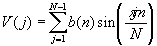
The transform of a real, odd sequence is a sine transform. A real odd vector is antisymmetric, that is, V(j) == -V(-j) or V(j) == -V(2N-j). As above, the vector V should be thought of as 2N points long, but here only the points V(j), j=1, ..., N-1, a total of N-1 points, need be given. This is true because we know that V(0) and V(N) are always 0 if the sequence is odd. Consequently, of the total 2N sequence, N-1 values are repeated twice and two are always 0. The sine transform is defined as,

The inverse FFT is given by,

Double Precision Complex FFT of Vector of Real Numbers

The forward Fourier transform is calculated as:

where X is the input vector of double precision real numbers and A is the output vector of double precision complex numbers.

The Inverse Fourier Transform is calculated as:

Math<Toolkit> provides a set of classes to generate forward and inverse fourier transformations. The classes provided are

           os_vec_dcomplex_fft          transformation of a vector of double complex numbers
           os_vec_dreal_fft                 transformation of a vector of double real numbers
           os_mat_dcomplex_fft          transformation of a matrix of double complex numbers
           os_vec_dreal_cosine_fft      cosine transformation of a vector of double real numbers
           os_vec_dreal_sine_fft         sine transformation of a vector of double real numbers

The example code below shows the usage of the above classes to generate fourier transformations.

Example <ospace/math/examples/doublefft.cpp>


  #include <ospace/math.h>


int
main()
  {
  os_math_toolkit math_init;

  double vec_data[ 5 ] = { 1, 2, 1, 3, 4 };
  os_num_vector< double > vec( 5 );

  for ( int i = 0; i < 5; i++ )
    {
    vec[ i ] = vec_data[ i ];
    }

  os_vec_dreal_fft fft;

  cout << "forward = \n" << fft.forward( vec ) << endl;
  cout << "inverse = \n" << fft.inverse( vec ) << endl;


  return 0;
  }